| <<Vol. 1 Table of Contents | |
|
|
|
|
2006 |
Volume 1, pp 53-76 |

Time, Place, and Content
Jonathon D. Crystal
University of Georgia
|
|
||||||||||||||||||||||||||||||||||
|
||||||||||||||||||||||||||||||||||
|
The ability to track events that unfold in time is a central problem in the life of an animal. Research on timing focuses on the mechanisms by which animals accomplish this temporal tracking. At the most basic level, timing research seeks to identify the psychological representation of time. The focus of this research is primarily experiments that examine the quantitative features of temporal anticipation, and it has yielded a rich assortment of theories that propose to account for these data. One limitation of this basic level of analysis is that it focuses on timing mechanisms in isolation. The ability to track an event in time is only useful to an animal if it can also integrate temporal information with other types of information. For example, a representation of when food will be available can produce general food-searching behaviors that will increase the likelihood of obtaining food. However, knowledge of where food will be available at a particular time may allow these food-searching behaviors to be directed at an appropriate location, thereby increasing the efficiency by which food is obtained. The focus of time-place learning is to identify the mechanisms by which temporal and spatial information is linked. Recently, research on temporal and spatial processing has been integrated with broader issues in memory research. This work focuses on time, place, and content (i.e., knowledge of what event occurred at a particular place and time). A central question in the discrimination of what-when-and-where (WWW) is the type of temporal representation that subserves this type of memory. The goal of this article is to integrate information about basic mechanisms of time perception (Time) with research on time-place learning (Time and Place) and research on the discrimination of WWW (Time, Place, and Content). The review of Time focuses on one of the quantitative features of temporal anticipation (the scalar property) and recent data that challenge this property. The review of Time and Place focuses on identifying the conditions under which different temporal mechanisms are used to discriminate time and place. The review of Time, Place, and Content focuses on identifying the timing mechanisms that may subserve the discrimination of WWW. Developments in basic research on time perception have implications for studying episodic memory (i.e., memories of when and where a specific event occurred). In particular, the review of Time below will include several lines of evidence which suggest that the psychological representation of time is nonlinearly related to physical estimates of time. These data prompt consideration of the proposal that interval timing is mediated by multiple, short-period oscillators. A multiple oscillator representation of time may be used to code the time of occurrence of events (Gallistel, 1990). In contrast, other representations of time, such as an elapsed interval, do not lend themselves to placing an event within a larger temporal context, such as it’s time of occurrence. Time-stamps for events, together with information about where the events occurred, may represent a promising direction for development of a quantitative, mechanistic theory of episodic memory in animals (i.e., memories of unique, personal past experiences). The validation of a behavioral model using animals may set the stage for the development of animal models of neural, molecular, and pharmacological mechanisms of episodic memory and disorders of memory (e.g., Alzheimer’s disease). Time Identifying an animal’s psychological representation of information in its environment is a fundamental issue in the study of comparative cognition (Roitblat, 1982). The temporal relation between events is a critical feature of the environment (Gallistel, 1990). Identifying the relation between psychological (i.e., subjective) estimates of time and physical estimates of time represents a powerful methodology for studying the representation of temporal information. The goal of this psychophysical approach is to identify a quantitative description of subjective estimates of time. The investigation of the psychophysical function for time has a long history of controversy (Nichols, 1891). Early psychophysical research suggested that the relation between subjective and physical estimates of time is best described by a power function with an exponent less than one (Eisler, 1976; Stevens, 1957). By contrast, later research suggested that the relation between psychological and physical time is linear (i.e., an exponent equal to one; Allan, 1983; Gibbon & Church, 1981). The linear timing hypothesis proposes that the subjective estimates of time are linearly related to physical time; linear timing is consistent with Weber’s law (i.e., the general property of sensory discrimination that the smallest stimulus-intensity difference that can be detected is a constant proportion of the comparison stimulus). Weber’s law may be documented by establishing that the standard deviation of time estimates is proportional to the mean of time estimates (i.e., a constant coefficient of variability, CV; Gibbon, 1977). By contrast, the nonlinear timing hypothesis proposes that the subjective estimates of time are nonlinearly related to physical time. The ability to estimate time allows an animal to adapt its behavior the temporal structure of its environment. An implication of nonlinear timing is that an animal is more proficient at adapting to some time periods and less proficient with other periods. An animal would gain a selective advantage over competitors (e.g., in foraging) if the animal was especially proficient at adapting to precisely the temporal structure of its environment, particularly if the environment is characterized by periodically available resources.
Linear timing The linear timing hypothesis may be evaluated by obtaining estimates of subjective time for a variety of target intervals. For example, in a fixed-interval (FI) procedure food is delivered contingent on the first response after a target interval has elapsed. Animals produce a characteristic break-run pattern of responses in individual trials (Schneider, 1969). The break-run pattern is characterized by withholding responses early in the trial, followed by a burst of responding that continues until food is received. The transition from a low to a high rate of responding is referred to as the start time. The data from individual trails are fit to a model of a low response rate followed by a high rate; the start time is defined as the time of transition from low to high rates that maximizes the goodness of fit. When many trials are aggregated, mean response rate increases as a function of time since the last reward. In a peak-interval (PI) procedure, discrete fixed-interval trials are mixed with non-rewarded trials that are typically much longer than the fixed interval (e.g., Roberts, 1981). On these long trials, animals produce a break-run-break pattern of responses (Cheng & Westwood, 1993; Church, Meck, & Gibbon, 1994). At some point after the start of the response burst, the animal stops responding (end time). The data from individual trials are fit to a model of a low response rate followed by a high rate and another low rate; the start and end times are defined as the transitions from low-to-high and high-to-low rates, respectively. When many trials are aggregated, mean response rate exhibits a peak centered on the target time.
Characteristics of performance in FI and PI procedures may be used to evaluate the relation between subjective and physical estimates of time (i.e., to construct a psychophysical function). An early example of linear timing by Dews (1970) appears in Figure 1. Dews examined the performance of pigeons in a FI procedure using 30, 300, and 3000 s. The figure shows measures of response rate plotted as a function of time into the target interval. The vertical axis represents response rate divided by the terminal rate, and the horizontal axis plots time divided by the fixed interval. Data from the three target intervals fall along the line in the figure, suggesting that performance from these conditions concur when the data are scaled in the proportional units used for the axes; the observation of agreement of experimental conditions when the data are expressed in proportional units is referred to as superposition. The data in Figure 1 are consistent with the hypothesis that the probability of starting to respond increases linearly with the fixed interval. An example of superposition from a PI procedure is shown in Figure 2. Rats were trained with 30, 45, or 60 s target intervals (Church, Lacourse, & Crystal, 1998). The figure shows response rate as a function of time in the top panel. These data are replotted in the middle panel using proportional measures (response rate divided by the maximum rate on the vertical axis and time divided by the reinforced interval on the horizontal axis). Note that the response distributions from the three conditions superimpose when plotted in proportional units. The start and end times from an analysis of individual trials are shown in the bottom panel of Figure 2. A major factor that contributes to the controversy over the psychophysical function for time is the number and spacing of target intervals. Studies that document superposition often use 2 or 3 intervals, often with a doubling or a ten-fold relation between successive target intervals. Three target intervals is the minimum number that can be used to evaluate the linear timing hypothesis. This number, together with a sufficiently wide spacing of target intervals, is adequate to compare a power function and a linear function (i.e., to identify the value of the exponent in a power function). However, it is inadequate to decide between linear and nonlinear timing hypotheses. Many studies in time estimation have been concerned with the generalized Weber function. For example, the relation between standard deviation and time estimates is constant followed by a linear increase according to a generalized Weber function (e.g., Fetterman & Killeen, 1992). According to this proposal, a single bend in an otherwise linear function is expected for intervals in the millisecond range. To evaluate a generalized Weber function, a few target intervals with increasing spacing as a function of interval conditions is appropriate because the single nonlinearity in the theoretical function is expected for the shortest intervals. However, this approach is less useful for testing nonlinearities that occur throughout the temporal range or that occur at unknown target intervals. Although the linear timing hypothesis predicts that measures of temporal performance are proportional to the target interval across a wide range of intervals, the hypothesis can be stated more precisely by focusing on two levels of analysis. Timing estimates consist of a linear component plus random error according to this more precise version of the linear timing hypothesis. When fitting a theoretical function to a data set, the residuals are the differences between the observed and expected values. The residuals are expected to be randomly distributed with respect to the theoretical function if the theoretical function provides an adequate description of the data. In contrast, the theoretical function is an inadequate description of the data if there is a systematic trend in the residuals. Therefore, the linear timing hypothesis can be specified at the level of mean performance and residuals. According to the most basic description of the linear timing hypothesis, psychological estimates of time are expected to increase as a constant proportion of physical estimates of time. According to the more detailed description of the linear timing hypothesis, the departures from the linear prediction are expected to be randomly distributed. Note that according to this argument, the critical issue is the putative existence of a systematic trend in the residuals rather than the relative size of linear and nonlinear components of the data. In the next section, data are presented to evaluate the more detailed description of the linear timing hypothesis. Nonlinear timing A small number of target intervals is adequate to evaluate the basic description of the linear timing hypothesis (cf. Figure 1 and bottom panel of Figure 2). However, many closely spaced interval conditions are required to evaluate the detailed description of the linear timing hypothesis. An efficient method for testing many closely spaced target intervals can capitalize on the observation that animals can track predictable changes in fixed-interval values across successive intervals (Church & Lacourse, 1998; Crystal, Church, & Broadbent, 1997; Higa, Wynne, & Staddon, 1991; Innis & Staddon, 1971; Ludvig & Staddon, 2005; Wynne, Staddon, & Delius, 1996). There is a growing body of recent research that suggests that the subjective estimate of time is nonlinearly related to physical time. Small departures from linearity have important theoretical implications. In the sections that follow, tests of the linear and nonlinear timing hypotheses are described from three domains: (a) the production of short intervals using modified FI and PI procedures, (b) the perception of short intervals using two-alternative choice procedures, (c) anticipation of daily (i.e., circadian) meals. This section concludes with a comparison of these data with earlier research in the literature. Nonlinearity in the production of short intervals A ramp procedure was designed to test the detailed description of the linear timing hypothesis (Crystal, Broadbent, and Church, 1997). Rats were trained to track a change in the target interval value. The ramp procedure is similar to a FI procedure in that the first response after the target interval is rewarded, at which point the next target interval begins. However, the target interval value changes across successive intervals in the ramp procedure. For example, for one group of animals, the target intervals examined were 20 to 150 s with a 2-s step size (i.e., permitting the assessment of 66 closely spaced target intervals). At the start of a daily session, the initial target interval and the direction (ascending or descending) were randomly selected for each rat. The target interval changed on successive trials until an endpoint in the range was reached, at which point the direction was changed. In summary, the target intervals changed in a predictable manner. For example, the sequence of target intervals might be 24, 22, 20, 22, 24 and 26 s etc. For a second group of rats, the intervals ranged from 30 to 160 s; in all other respects, the procedure was identical for the two groups. These data were reported as Experiment 1 of Crystal et al., 1997) and are reproduced here in Figure 3. The top left panel of Figure 3 shows start times plotted as a function of the target intervals for both groups. Start times increased as a function of target intervals in an approximately linear fashion. These data are replotted as residuals in the bottom left panel of Figure 3. Note that the data are the same in the two left panels of Figure 3, with the only difference being the removal of the linear trend. This plot reveals a surprisingly systematic trend in the residuals for both groups, given the original plot of start times. The systematic trend represents an empirical conflict with the linear timing hypothesis. Although the observed nonlinearities are small relative to the approximately linear increase in start times, the nonlinearities are sufficiently robust to be reliably detected. Therefore, the observed nonlinearities, although relatively small, may provide information about the underlying representation of time.
Two overlapping ranges of intervals were compared to establish that the nonlinear data from the ramp procedure documents characteristics of the intervals being timed rather than a range effect. The range in common between the groups (30-150 s) was examined to identify the variable that controlled the linear and nonlinear trends. There are two potential controlling variables: (a) the specific target interval or (b) the position of the interval within the range of intervals. Figure 3 shows the start times and residuals for the two groups of rats. Start times and residuals each superimposed across the groups when the data were plotted as a function of intervals (left panels). When the start times and residuals were plotted as a function of the percentage of the range, data from the two groups were displaced from one another (i.e., the data from the groups did not superimpose; right panels). These data suggest that the nonlinearities are characteristics of timing specific target intervals and represent an empirical conflict with the linear timing hypothesis. It is noteworthy that in this experiment all aspects of the procedure were carefully controlled so that the only variable that differed between the two groups was the range of intervals. This approach provided a within-experiment assessment of the relative influence of timing specific target intervals and a range effect. The observation that the same pattern of residuals was replicated in the two groups strongly suggests that the nonlinearities are associated with timing specific target intervals. The ramp procedure described above is similar to a FI procedure in that the animal stops responding when it obtains food. Consequently, it is possible to use start times as an estimate of when the animal expects food to occur, but it is not possible to estimate when an animal would give up responding after the target interval has elapsed. In contrast, the PI procedure permits an estimate of both start and end times, and patterns of start and end times have been useful in identifying the type of mechanism responsible for timing (Cheng & Westwood, 1993; Cheng, Westwood, & Crystal, 1993; Church et al., 1994; Gibbon & Church, 1990).
The ramp procedure was modified by randomly inserting 660-s fixed intervals occasionally into the sequence of ascending and descending intervals within the range of 10 to 140 s in order to examine the pattern of start and end times. The probability of a 660-s trial ranged from .10 to .15. Because the 660-s trials were inserted into the sequence of ramp trials, the next interval in the sequence occurred after a long (i.e., 11 min) delay. For example, the sequence of target intervals might be 16, 14, 660, 12, 10, and 12 s. These data were reported as Experiment 2 in Crystal et al. (1997) and are reproduced in Figures 4 and 5. Figure 4 shows start times for target intervals that ranged from 10 to 140 s. Figure 5 shows start and end times from 660-s trials plotted as a function of the previous interval in the sequence (i.e., plotted as a function of intervals between 10 and 140 s). Note that start and end times both exhibit systematic departures from linearity. Importantly, the start and end residuals superimpose; the implication of superimposition of residuals will be discussed below. It is likely that the 11-min delays inserted into the sequence of ascending and descending target intervals influences the precision with which quantitative parameters of the data may be estimated (e.g., locations of local maxima and minima); 11-min delays between successive target intervals represents a significant retention interval, which limits between-experiment comparisons of residuals. Nevertheless, the data suggest that the rats tracked the changing target intervals and that the method was adequate to compare start and end times (i.e., a within-experiment comparison).
The observation that start and end residuals superimpose constrains the type of proposals that may explain the nonlinearities. The similarity of start and end residuals can be used to infer the source of nonlinearities in timing. Two sources will be considered. First, nonlinearities may indicate that the representation of times in memory is systematically distorted (memory representation). Second, nonlinearities may reflect distortions in the process that governs the decision to respond (decision processes). It may be helpful to consider the decision to respond on an individual trial as a comparison between an estimate of an elapsing interval (current time) and a memory of the target interval (remembered time); responding occurs when the two representations (current and remembered times) are sufficiently similar using a decision threshold (Gibbon, Church, & Meck, 1984). Figure 6 illustrates the predicted pattern of temporal behavior if nonlinearities are introduced in the memory representation of time (left panels) or in a decision process (right panels). Nonlinearity in memory (left panels of Figure 6) means that some target intervals are remembered as relatively short and other intervals are remembered as relatively long. Systematic variability in the durations stored in memory produces bursts of responding (start, middle, and end times) that occur early for some target intervals and late for other intervals (top left panel of Figure 6); the middle is half-way between the start and end times. Remembered durations that are relatively short produce early starts, middles, and ends. Remembered durations that are relatively long produce late starts, middles, and ends. Note that systematic variation in the durations stored in memory produces departures from linearity that superimpose for start and end times (bottom left panel of Figure 6).
In contrast, nonlinearity in the decision process (right panels of Figure 6) means that the decision threshold is relatively strict for some target intervals and relatively lenient for other intervals. Systematic variability in the decision threshold produces bursts of responding that are wide for some target intervals and narrow for other intervals (top right panel of Figure 6) depending on how strict is the decision threshold; note also that the middle times are linear according to this proposal. A strict threshold produces a narrow burst of responding, meaning that the start time is late and the end time is early. A lenient threshold for responding produces a wide burst of responding, meaning that the start time is early and the end time is late. Note that systematic variation in thresholds produces departures from linearity that do not superimpose for start and end times. Instead, the start and end residual patterns are predicted to be 180° out of phase if the decision process is not linear (bottom panel of Figure 6). In conclusion, the nonlinear patterns in start and end times can be used to infer the source (memory representation or a decision process) of nonlinearities in timing. The observation that start and end residuals superimpose (Figure 5) suggests that some intervals are remembered as relatively long and other intervals are remembered as relatively short; i.e., the nonlinearity occurs in the memory representation of time. The data rule out the hypothesis that some intervals are timed with relatively strict vs. lenient decision thresholds (Crystal et al., 1997). Nonlinearity in the perception of short intervals
The data shown in Figures 3, 4, and 5 document nonlinearities in the production of time intervals (burst of responses in variations of fixed-interval procedures). Nonlinearities in the timing of behavior may reflect nonlinearities in the central processing of time, or alternatively, it may reflect nonlinearities in the motor output of behavior. A critical way to test these alternatives is to examine measures of sensitivity to time using a discrimination procedure. In a two-alternative discrimination procedure, a stimulus duration is presented and the animal gives one of two responses (e.g., press left or right lever) to classify the duration as short or long. Motor output is relatively low (a single classification response) in discrimination tasks, in contrast to a burst of responses in FI procedures; moreover, motor output is constant in short and long conditions. Figure 7 shows a measure of sensitivity to time from a discrimination procedure using many closely spaced inter-interval conditions. Sensitivity to time is characterized by multiple local maxima (Crystal, 1999, 2001b). The procedure involved presenting a short or long noise followed by the insertion of two levers. Left or right levers were designated as correct after short or long stimuli. For each short duration, accuracy was maintained at approximately 75% correct by adjusting the duration of the long signal after blocks of discrimination trials. This titration procedure resulted in a long duration approximately 2 to 2.5 times the short duration. Sensitivity to time was measured using signal detection theory (Macmillan & Creelman, 1991). Sensitivity to time was approximately constant for short durations from 2 to 34 s. However, local peaks in sensitivity to time were observed at approximately 12 and 24 s (left and middle panels of Figure 7). Local peaks in sensitivity to time were observed at 0.3 and 1.2 s when short durations in the millisecond range were tested (right panel of Figure 7). Multiple local maxima in sensitivity to time represent an empirical conflict with the linear timing hypothesis. The ability to directly compare nonlinearities in the ramp and titration procedures is limited by relatively little overlap in the interval conditions. The data reviewed in this section suggest that the psychological representation of time is nonlinearly related to physical estimates of time. A nonlinear representation of time is consistent with the proposal that interval timing is mediated by multiple, short-interval oscillators. Multiple oscillators may be used to represent the time of occurrence of unique events. The interpretation that nonlinearities in sensitivity to time are based on short-period oscillators is tested in the next section by examining sensitivity to time 24 hr (i.e., sensitivity near a circadian oscillator).
Nonlinearity in the timing of 24 hr One interpretation of the data in Figure 7 is that each local maximum in sensitivity to time identifies the period of an oscillator. According to this proposal, short-period oscillators mediate short-interval timing in ways that are similar to how a circadian oscillator mediates timing near 24 hr. If the hypothesis that local maxima in the millisecond to second range identify short-interval oscillators is correct, then a local maximum in sensitivity to time is predicted to occur near 24 hr for circadian timing (i.e., near the well-established circadian oscillator, e.g., Mistlberger, 1994). A series of experiments investigating meal anticipation was undertaken to test the hypothesis that a circadian oscillator is characterized by a local maximum in sensitivity to time (Crystal, 2001a); alternative hypotheses about the mechanisms involved in meal anticipation are reviewed by Gallistel (1990) and Mistlberger (1994). Figure 8 shows anticipation functions for intermeal intervals near the circadian range (22 to 26 hr) and outside this range (14 and 34 hr). The data were obtained by restricting daily food availability to 3-hr meals, which rats earned by breaking a photobeam in the food trough. The rats inspected the food trough before meals started, with response rates increasing later into the interval for intermeal intervals near the circadian range than for intervals outside this range (Figure 8). Sensitivity to time was estimated by the spread of the response distributions. The spread was smaller (i.e., lower variability) for intermeal intervals near the circadian range than for intervals outside this range, as shown in Figure 9. The data in Figure 9 document a local maximum in sensitivity to time near 24 hr. The local maximum in sensitivity to time near 24 hr is consistent with the hypothesis that a property of an oscillator is improved sensitivity to time.
The conclusion that emerges from the series of experiments
evaluating sensitivity to time is that multiple local
maxima in sensitivity to time are observed in the discrimination
of time across several orders of magnitude (Figure
10; Crystal, 1999, 2001a, 2001b). The existence of a local
maximum near a circadian oscillator (Figure 10, peak on
right side) and in the short-interval range (Figure 10, peaks
on left side) are consistent with timing based on multiple oscillators
(Church & Broadbent, 1990; Crystal, 1999, 2001a,
2003, in press b; Gallistel, 1990). According to multiple
oscillator proposals, each oscillator is a periodic process that
cycles within a fixed amount of time; an oscillator is characterized
by its period (i.e., cycle duration) and phase (i.e.,
current point within the cycle). Each unit within a multiple
oscillator system has its own period and phase. Therefore, a multiple oscillator system includes several distinct periods.
Sensitivity to time an interval near an oscillator is expected
to be higher than timing an interval farther away from the
oscillator. Therefore, multiple local maxima in sensitivity to
time across several orders of magnitude (Figure 10) suggest
the existence of multiple short-period oscillators.
Comparisons with literature The sections above reviewed three lines of evidence that conflict with the linear timing hypothesis despite numerous reports in the literature favoring the linear timing hypothesis. Documenting a different empirical description of the psychophysical properties of time leads to a basic question about the timing literature: Why were nonlinear patterns not observed previously? One explanation focuses on the number and spacing of target intervals. As discussed above, a small number of widely spaced target intervals has traditionally been examined. Although this approach is adequate to evaluate a linear trend across a wide range, it is not well suited to examining systematic trends in residuals. This problem can be illustrated by selecting a subset of the ramp-procedure data using a number and spacing of conditions that is typical of the timing literature. The left panel of Figure 11 shows start times plotted as a function of four intervals that were selected from the larger data set that appears in Figure 3. The residuals for this subset of data appear in the right panel of Figure 11. Although there is a nonlinear trend in the original data set consisting of many, closely spaced target intervals (Figure 3), it is not possible to detect this trend in the small subset in Figure 11. In this case, using a few widely spaced intervals leads to a conclusion that is at variance with the conclusion that emerges from the larger data set. Consequently, the timing literature has been interpreted as providing evidence for linear timing, in part, because the literature did not provide an adequate number and spacing of interval conditions. Therefore, the observation of a systematic nonlinear pattern in Figures 3, 4, and 5 using different procedural and quantitative methods does not reflect a data conflict with the published literature. In the case of measures of sensitivity to time, large collections of interval conditions have been selected from many studies. Typically these data have been presented as scatter plots, which visually feature the overall trend of many data points rather than residuals. However, these scatter plots can be used to evaluate the published literature for evidence of local maxima in sensitivity to time. For example, Gibbon, Malapani, Dale, and Gallistel (1997b) plotted the coefficient of variability (CV; standard deviation of time estimates divided by the mean of time estimates) as a function of target intervals using 43 data sets from the literature (Figure 3 in their article). I have replotted their scatter plot in the top panel of Figure 12 using a reverse-ordered vertical axis so that high points in the figure correspond to high sensitivity to time. To examine the shape of the sensitivity function, the data from Gibbon et al were averaged in two-point blocks and subjected to a 3-point running median. These data appear in the bottom panel of Figure 12. Sensitivity to time using Gibbon’s selection of data from the literature is characterized by multiple, local maxima. The middle of the local maxima in the bottom panel of Figure 12 occurs at approximately 0.2, 0.3, 1.2, 10, and 20 s. Clusters of relatively high points near these intervals can also be seen in the top panel of Figure 12. The values of local maxima derived from Gibbon’s selection of data are strikingly similar to local maxima that were observed in Figure 7: 0.3, 1.2, 12, and 24 s (Crystal, 1999, 2001b, 2003). Although the shapes of the sensitivity function in Figures 7 and 12 differ, the similarity in the locations of local maxima is noteworthy given that the data in Figure 12 come from 43 different data sets. Importantly, the data that appear in Figure 12 were independently selected by Gibbon et al; consequently, the selection of experiments for inclusion in the figure cannot be responsible for the observed local maxima. The quantitative similarity between the observed locations of local maxima in sensitivity provides an independent, converging line of evidence which suggests that sensitivity to time is nonlinear. In addition, averaging the data to obtain a single function, rather than a scatter plot, is important for evaluating nonlinearities. The main barrier in evaluating a local maximum near 24 hr is the generally accepted view that food-anticipatory activity to a daily meal develops only when the interval between successive meals is near 24 hr. Although it is generally accepted that animals cannot anticipate intermeal intervals outside a limited range near 24 hr (Aschoff, von Goetz, & Honma, 1983; Boulos, Rosenwasser, & Terman, 1980; Madrid et al., 1998; Mistlberger & Marchant, 1995; Stephan, 1981; Stephan, Swann, & Sisk, 1979a, 1979b; White & Timberlake, 1999), this conclusion is based on a relatively limited data set. I reexamined the published data from long intermeal intervals that are substantially less than 24 hr in experiments that used behaviors that are instrumental in producing food (e.g., approaching the food source or pressing a lever). Figure 13 shows a reanalysis of 18 and 19 hr intermeal intervals (Bolles & Stokes, 1965; Boulos et al., 1980) together with 14-hr data from Crystal (2001a); the reanalysis also included a 24-hr condition from each experiment. The temporal function for intervals below the circadian range is less steep and has lower terminal response rates than intervals in the circadian range. However, these features are characteristic of relatively high variability (i.e., low sensitivity to time), which is consistent with the data in Figure 8 (Crystal, 2001a). By contrast, wheel-running activity does not precede meals at these intervals (Bolles & de Lorge, 1962; Bolles & Stokes, 1965; Mistlberger & Marchant, 1995; Stephan et al., 1979a; White & Timberlake, 1999). Therefore, behaviors that are instrumental in producing food may represent a more sensitive measure of food anticipation than measures of general activity.
In conclusion, the answer to the question “Why were nonlinear patterns not observed previously?” has different answers in the three cases reviewed. In general, the literature has not traditionally evaluated many closely spaced interval conditions. When large numbers of conditions have been selected from multiple experiments, the evidence for local peaks in sensitivity to time may be overlooked by relying on scatter plots. The conclusion that long intervals (14-19 hr) cannot be timed is based on the high variability in these response distributions. Implications for theories of time One interpretation of local maxima in sensitivity to time is that time perception is mediated by multiple oscillators. The location of a local maximum can be used to identify an oscillator’s period. According to this proposal, short-interval timing in the range of milliseconds to seconds is characterized by several oscillators (e.g., 0.2-0.3, 1.2, 10-12, 20-24 s). The hypothesis that local peaks in sensitivity identify the period of an oscillator led to the prediction that a peak in sensitivity to time would be documented near 24 hr, a prediction that was confirmed (Figure 9; Crystal, 2001a). A central feature of a multiple-oscillator theory of timing is a nonlinear representation of time. Two multiple-oscillator theories of timing have been proposed. Church and Broadbent (1990) proposed that elapsed time is represented by the phase of a set of oscillators, each with a unique period (e.g., 100, 200, 400, 800 msec, etc). The representation of elapsed time increases nonlinearly as a function of time. Information about the phase of the oscillators at the time of reward is stored in reference memory (i.e., reference memory consists of a correlation matrix indicating the degree of association between the oscillators). The status of the oscillators during a timing episode is compared with the reference-memory representation of the rewarded duration, rendering a decision to respond or not to respond. Gallistel (1990) proposed that estimates of the time of occurrence of events are mediated by multiple oscillators, each with a unique period. According to this proposal, the occurrence of an event does not ‘reset’ the timing mechanism. Instead, the oscillators were proposed to run throughout the life of the organism. Consequently, the status of a series of oscillators provides a unique representation, or time stamp, for the occurrence of an event. Moreover, Gallistel proposed that animals store three types of information in memory when a significant biological event occurs: time of occurrence, spatial co-ordinates, and information about the quality (or content) of the event. According to Gallistel’s proposal, the calendar-date system of biological oscillators, together with spatial and content information, allows the organism to extract patterns or correlations among events (e.g., Pavlovian conditioning). Integration of research from interval and circadian timing Efforts to understand the ability to track temporal regularities in the environment have developed along two relatively independent paths, one focusing on timing short intervals and the other focusing on timing intervals of approximately a day. These efforts have used different experimental manipulations and dependent variables, constructed different theoretical frameworks, and communicated findings to different research communities. These factors have led to the conclusion that short-interval timing and circadian rhythms are based on unrelated mechanisms. It is important to subject these conclusions to empirical tests. Below I summarize tests that are relevant to developing a theory of timing that encompasses the discrimination of temporal intervals across several orders of magnitude – from milliseconds to days. The resetting characteristic of the timing mechanism is a critical feature that distinguishes a pacemaker-accumulator from a circadian oscillator. In particular, an oscillator is endogenous and self-sustaining. A defining feature of a circadian oscillator is that periodic output from the oscillator continues without additional periodic input. Consequently, an oscillator is only partially affected by the presentation of an environmental reset cue. The circadian system requires several days of environmental input before the system is set to a new local time, which leads to the familiar experience of jet lag. By contrast, a hallmark feature of a short-interval clock is that it estimates the elapsed time between the presentation of arbitrary events, as in the case of a stopwatch (Church, 1978); the elapsed time since the arbitrary event is represented by the number of pulses accumulated from a pulse-emitting pacemaker (referred to below as a pacemaker- accumulator mechanism). Presentation of the to-be-timed event is presumed to reset the representation of elapsed time. Consequently, a pacemaker-accumulator is completely affected by the presentation of an environmental reset cue. Figure 14 shows an example of a phase-shift manipulation applied to short-interval timing. A pacemaker-accumulator mechanism predicts complete adjustment on the initial interval after a phase shift on the assumption of complete reset (Gibbon, Fairhurst, & Goldberg, 1997a), whereas an oscillator mechanism predicts initial incomplete adjustment to a phase shift. Rats were trained with a 100-s FI procedure. An early, free food pellet was provided to implement a phase shift. Four food cycles were required before adjustment was complete, which is consistent with an oscillator mechanism of short-interval timing of 100 s.
A defining feature of a circadian oscillator is that periodic output continues after the termination of periodic input. For example, when animals are entrained by the presentation of a daily meal, the anticipation of the meal continues for more than one cycle when multiple meals are omitted (e.g., Boulos et al., 1980; Escobar, Díaz-Muñoz, Encinas, & Aguilar- Roblero, 1998). In contrast, a defining feature of a pacemaker- accumulator system is that elapsed time is measured with respect to the presentation of a stimulus (Gibbon et al., 1997a). Consequently, the output of a pacemaker-accumulator system is periodic only if presented with periodic input. Periodic output from a pacemaker-accumulator is expected to cease if the periodic input is discontinued. Therefore, the hypothesis that the timing of short and long intervals is based on a pacemaker-accumulator or oscillator mechanism can be assessed by discontinuing periodic input (i.e., extinction) and assessing subsequent anticipatory behavior. When rats received meals with an intermeal interval of 16 hr, they anticipate the arrival of the meal. After discontinuing the periodic delivery of meals (i.e., extinction), behavior was periodic in the absence of additional periodic input (Crystal, in press a). Similarly, when rats were trained with a 96-s FI procedure, they anticipated the arrival of food. After discontinuing the periodic delivery of food, behavior was periodic in the absence of additional periodic input (Crystal, 2005). Testing for the use of a self-sustaining, endogenous oscillator to time short and long intervals may contribute to the development of a unified theory of timing that encompasses the discrimination of temporal intervals from milliseconds to days. Oscillators may also be used as the timing mechanisms in time-place discrimination and the discrimination of what, when, and where. An interval or oscillator representation of time may provide a basis for anticipating the arrival of food at specific places (time-place discrimination). A multiple-oscillator system is a mechanism that could provide a unique time-stamp that subserves the discrimination of WWW (i.e., memory for what event occurred at a particular time and place). In the sections that follow, research on timing mechanisms is applied to two domains: time-place discrimination and the discrimination of what, when, and where. Time and Place The review of Time and Place focuses on identifying the conditions under which different temporal mechanisms are used to discriminate time and place. In most situations, multiple cues are available to solve a time-place discrimination. Consequently, it is necessary to separately evaluate the contribution of each available mechanism. The availability of resources is sometimes correlated with time of day. For example, oystercatchers anticipate the tidal rhythms that determined mollusk availability on tidal mud flats (Daan & Koene, 1981). Biebach and colleagues (Biebach, Gordijn, & Krebs, 1989; Krebs & Biebach, 1989) developed a method to study time-place learning in a laboratory environment. Food was available in one of four rooms in a fixed sequence each day (e.g., rooms A, B, C, and D). Food availability in each room was determined based on time of day (e.g., 0600 to 0900 in room A, 0900 to 1200 in room B, etc.). In these experiments, garden warblers restricted most of their visits to the temporally correct feeding rooms. However, the observation that an animal searches for food at the appropriate time of day does not necessarily indicate that the animal is using time of day as a cue in time-place discrimination. The inability to draw this conclusion stems from the availability of alternative solutions to the discrimination problem. Multiple mechanisms to solve time-place discrimination The availability of multiple mechanisms to solve a time-place discrimination may be illustrated with the following example. Food is available for a limited period of time in the morning (time 1), afternoon (time 2), and evening (time 3), at locations A, B, and C, respectively. An animal may learn to visit each location at the appropriate time of day. Although the availability of food may be described in terms of time of day, as in the above example, there are four mechanisms that may be used to solve the discrimination. First, a win-stay lose-shift strategy could solve the discrimination. An animal could search randomly until it found food at location A, continue to exploit location A until food there becomes scarce, at which point it would begin to search new locations until it consumes food at locations B and C. Although an animal using this strategy would produce behavior that is correlated with time of day, the animal would not need to have a representation of time of day. Second, a representation of the order of locations could be used without any temporal information. Carr and Wilkie (1997a, 1997b) proposed that animals may use an ordinal representation of time to solve time-place discriminations. According to this proposal, locations A, B, and C are represented as first, second, and third of the day. If there are two locations per day, an alternation strategy is a simpler version of this strategy that does not require circadian information (i.e., visit location A after B and location B after A, effectively alternating between locations A and B). Third, an interval-timing mechanism may be used to solve the discrimination (i.e., a pacemaker-accumulator mechanism reset by an environmental event). For example, an animal may time the interval between successive locations using food at each location as a reset event; alternatively, a single event in the day (e.g., a light-cycle transition) may reset the interval-timer, in which case the availability of food at each location is correlated with one of three elapsed cumulative intervals. Fourth, a representation of time of day may be used to solve the discrimination. For example, arrival at the temporally correct location could be based on an oscillator entrained to daily light cycles or food cycles (Mistlberger, 1994). The sections that follow review time-place experiments in which each of the above mechanisms are tested. This review is concluded with a section that summarizes the conditions under which different temporal mechanisms are used to discriminate time and place. Time-place discrimination using short intervals Carr and Wilkie (1998) developed a short-interval time-place discrimination. Food was available during each of four successive segments of time at each of four locations in a box using a fixed association between time segments and locations. For example, a rat might earn food for four minutes at lever 1, followed by additional four minute segments at each of levers 2, 3, and finally 4. Carr and Wilkie compared groups of rats that received 4-, 6-, or 8- min segments. The rats restricted most of their responses to the correct lever at the appropriate time. The variability in the distributions of response rates as a function of time was constant at each lever. Similarly, the precision with which the rats switched from one lever to the next was constant as the session progressed. Finally, the response distributions superimposed when plotted in relative time (i.e., elapsed time divided by 4, 6, or 8 min for the three groups, respectively); however, when a rat must discriminate two different intervals within a sequence of four locations, the data do not superimpose in a short-interval time-place task (Crystal & Miller, 2002). Carr and Wilkie’s data suggest the use of an interval-timing mechanism to time successive intervals, rather than timing one interval equal to the length of the session.
Carr and Wilkie’s (1998) experiment randomly tested rats daily in a random order within a 3-hr window of time. Therefore, time of day was rendered irrelevant, which limits the conclusion that interval (rather than circadian) timing mediates short-interval time place discrimination. An alternative approach is to make both interval and circadian timing mechanisms available by testing the animals at the same time each day. If both time-of-day and interval-timing mechanisms are available, tests can be designed to identify which mechanism the animal uses to restrict its visits to the correct locations and times. This feature has generally not been included in previous time-place experiments. Pizzo and Crystal (2004b) trained rats with multiple cues available (i.e., confounded) and proceeded to separately unconfound each cue. Daily 56-min sessions were divided into eight 7-min time zones. During each time zone a different location on an eight-arm radial maze provided food using a sequence that was randomly determined for each rat before the start of the experiment. The rats obtained multiple pellets within each time zone by leaving and returning to the correct location. The rats restricted most of their visits to the active location during each time zone (Figure 15). A win-stay lose-shift strategy without any knowledge of time or place was ruled out from the following observations. The rats (a) anticipated locations before they became active, (b) anticipated the end of the currently active locations, and (c) discriminated currently active locations from earlier and forthcoming active locations in the absence of food transition cues. After the rats had left the previously active location, they visited the next correct location more often than would be expected by chance in the absence of food transition cues. A series of experiments that manipulated the time at which (a) the colony lights were turned on, (b) the animals were placed in the maze, and/or (c) the doors to the arms of the maze were opened led to the conclusion that the rats used handling or opening doors as a cue to visit the first location and timed successive 7-min intervals to get to subsequent locations. Time place discrimination using long intervals Carr and Wilkie (1997a, 1997b; Carr, Tan, & Wilkie, 1999) argued that rats’ performance in time-place tasks is in part based on an ordinal representation of time. When rats were trained to press one lever in the morning and another lever in the afternoon, the impact of skipping a test session depended on time of day; when the morning session was skipped and a test occurred in the afternoon, the rats incorrectly lever pressed at the morning location, but when the afternoon session was skipped and testing occurred the next morning, the rats lever pressed at the morning location (Carr & Wilkie, 1997b). Carr and Wilkie argued that these results imply an ordinal representation of time because in both cases the animals started daily testing by going to the first location of the day. According to this proposal, the rat resets its ordinal timer each day by consulting a circadian oscillator and visits specific locations by consulting an ordinal timer. Representations on an ordinal scale of measurement capture only the order of values on the ordinal scale. For example, finalists in a race may be ranked first, second, and third (an ordinal scale), and this measurement conveys no information about how close were the finish times among the finalists. A higher order representation using an interval or ratio scale would be required to permit additive and multiplicative transformations, respectively (Stevens, 1951). Pizzo and Crystal (2002) tested a prediction of an ordinal representation of time. In particular, if an animal uses an ordinal scale of measurement, it should be insensitive to transformations that require a higher order scale. Consequently, an animal using an ordinal scale should be insensitive to an additive transformation. Rats searched for food twice in the morning and once in the afternoon (group AB-C) or once in the morning and twice in the afternoon (group A-BC) using three locations (A, B, and C). To produce an additive transformation, the time of the middle search (B) was shifted late (for group AB-C) or early (for group A-BC) on nonrewarded probes. Because an ordinal representation of time is insensitive to an additive transformation, changing the relative position of B (i.e., early or late) should have no effect; an ordinal mechanism represents the temporal order of events (i.e., B is second) but does not represent the relative temporal placement of events (i.e., that B is temporally closer to A than to C). The rats visited location B at chance when the B shift was conducted unusually early or late, contrary to an ordinal mechanism. When the posttesting meal and lightdark transitions in the colony were omitted, the rats visited correct locations with impaired performance but at above chance levels on nonrewarded probes. These data are consistent with interval and circadian representations of time. Pizzo (2005) undertook a series of experiments to separately unconfound multiple timing mechanisms in daily time-place discriminations using long intervals between two daily meals. Presumably, the spacing between two daily meals would influence the type of mechanism (i.e., circadian or interval timing) used to anticipate a meal. In addition, the availability of nontemporal cues (e.g., handling) may influence the use of nontemporal (e.g., alternation) strategies. In one experiment, the rats were placed on a T-maze twice per day with 7 hr between the two daily shifts. Food was available in one location in the morning and the other location in the afternoon. The rats solved the time-place discrimination using an alternation strategy (Pizzo & Crystal, 2004a). For example, when the morning shift was skipped, the rats visited the location appropriate for the morning when they were later tested in the afternoon. Similarly, when the afternoon shift was skipped, the rats visited the location appropriate for the afternoon when they were next tested in the morning. When a phase advance of the light cycle was conducted (i.e., light onset in the colony occurred earlier than usual), the rats visited the location appropriate for the morning shift. These data suggest that the rats used an alternation strategy to meet the temporal and spatial contingencies of the time-place task (Pizzo & Crystal, 2004a). The handling of the rats prior to testing in each shift may have facilitated the use of an alternation (i.e., nontemporal) strategy. To investigate the conditions under which circadian and interval-timing mechanisms are used in time place discrimination, the temporal spacing of two daily meals was manipulated (Pizzo & Crystal, in press). Rats earned the first daily meal by pressing a lever in an operant box beginning 3.5 hr after the start of a session and a second daily meal by pressing another lever. The second meal started 0.75, 1.75, 3, or 7 hr after the start of the first meal, using independent groups of rats. Two types of manipulations were used. First, occasionally a meal was omitted and performance immediately prior to the next meal was evaluated to assess the use of an alternation strategy. Second, the time at which the test session started was adjusted so that the first meal within the session would be scheduled to start at the time of day at which the second meal usually started. By putting into conflict time since the start of the session (i.e., an interval mechanism) and time of day (i.e., a circadian mechanism), the relative control of interval and circadian mechanisms was evaluated. When the meals were widely separated (3 or 7 hr between meals), approximately half of the rats used an interval-timing mechanism, and the other half used a circadian mechanism. When the meals were more closely spaced (0.75 or 1.75 hr), the rats timed two intervals, one from the start of the session until the first meal and the other from the first to the second meal. These data suggest that the resolution of a circadian mechanism is between 1.75 and 3.5 hr, and an interval timing mechanism can be used to time intervals from 0.75-7 hr (Pizzo & Crystal, in press). Interpretation A circadian representation of time provides information about daily events. However, other cues apparently compete with circadian information. For example, when salient nontemporal cues (e.g., handling the animals before each opportunity to earn food) occur at constant times of day, the rats used the nontemporal cue rather than time of day. When two large meals were predicted by time of day, a circadian mechanism was used when the meals were widely separated (3-7 hr). However, an interval timing mechanism was also used to anticipate these daily meals. When the meals were moved closer to one another, there was no evidence for use of a circadian mechanism; rather, the rats relied on an interval timing mechanism. In conclusion, although interval timing has typically been applied to the seconds to minutes range, the flexibility of interval timing appears to be considerable, ranging from very short intervals to at least 7 hr; to estimate an upper limit for an interval-timing mechanism, it will be necessary to test intervals above 7 hr. In conclusion, it is necessary to explicitly test for each mechanism rather than relying on the assumption that some timing mechanisms are used for short intervals and others are used for daily events. This conclusion motivates the need to evaluate multiple timing mechanisms in the discrimination of time, place, and content. Time, Place, and Content Tulving (1972) proposed a distinction between semantic and episodic memory. Semantic memory consists of factual knowledge about the world, whereas episodic memory consists of unique, personal, past experiences. Tulving’s (1972) classic definition is: “Episodic memory receives and stores information about temporally dated episodes or events, and temporal-spatial relations among these events.” (p.385). According to this definition, episodic recall involves retrieval of information about three aspects of an event or episode: what occurred, when did it transpire, and where did it take place (what-when-where, WWW). Tulving (1983) argued that episodic memory involves a recollective experience (i.e., conscious awareness that an event happened in the past). The hypothesis of cognitive time travel involves traveling back in time to re-experience an event (retrospective cognitive time travel) and traveling forward in time to anticipate or plan for the future (prospective cognitive time travel). Humans cognitively travel backward from the present by remembering personal, past experiences (episodic memory) and forward from the present by anticipating future needs (future planning; e.g., Tulving, 2002). Tulving (1985, 1993, 2002) has argued that cognitive time travel requires a sense of subjective time, autonoetic awareness (i.e., personal awareness), and a sense of self. Consequently, Tulving (1983, 2002, 2005; Tulving & Markowitsch, 1998) argued that cognitive time travel is unique to humans. Tulving (1983) opens Elements of Episodic Memory with: “Remembering past events is a universally familiar experience. It is also a uniquely human one.” (p. 1). Suddendorf and Corballis (1997) argued that “animals other than humans cannot anticipate future needs or drive states and are therefore bound to a present that is defined by their current motivational states” (p. 150; Bischof-Kohler hypothesis). Similarly, Roberts (2002) argued that animals are stuck in time. Clayton and colleagues (Clayton, Bussey, Dickinson, 2003a; Clayton, Bussey, Emery, & Dickinson, 2003b) distinguish between phenomenological and behavioral criteria. Definitions of cognitive time travel in terms of the conscious experiences that accompany recollection and planning (e.g., Tulving, 1983, 2002; Tulving & Markowitsch, 1998) represent an intractable barrier to the development of an animal model (Griffiths, Dickinson, & Clayton, 1999) because phenomenology cannot be evaluated in non-verbal animals. Clayton’s behavioral criteria focus on Tulving’s (1972) original definition: what occurred, when did it transpire, and where did it take place (i.e., on behaviors that can be evaluated in non-human animals). Clayton et al. (2003a) refer to memory that meets the following behavioral criteria as ‘episodic-like’ memory: (1) “Content: recollecting what happened, where and when on the basis of a specific past experience.” (2) “Structure: forming an integrated ‘whatwhere- when’ representation.” (3) “Flexibility: episodic memory is set within a declarative framework and so involves the flexible deployment of information.” (p. 686).
Clayton and Dickinson (1998) provided the first evidence of discrimination of WWW in food-storing scrub jays. They provided jays with the opportunity to cache either peanuts followed by wax worms or, on other trials, worms followed by peanuts and to retrieve the cached foods after either a short or long retention interval (RI). For some birds, the worms were decayed after the long RI, and for other birds they were replenished with fresh worms (peanuts did not decay). The birds preferred the worm rather than peanut cache sites when the worms were fresh, but reversed this preference when the worms were decayed. These data suggest that the jays are sensitive to what (food type), when (time of caching and recovery), and where (location in the tray). Since this initial demonstration, Clayton and colleagues have established a growing body of research to indicate that scrub jays have a detailed representation of what, when, and where food was cached. For example, jays (1) remember the specific food types that they cache and recover (Clayton & Dickinson, 1999a, 1999c), (2) remember the relative time and location of caches (Clayton & Dickinson, 1999c), (3) form integrated memories for the location and time of caching of particular foods (Clayton, Yu, & Dickinson, 2001), and (4) flexibly update information about caching episodes with new information acquired during the RI (Clayton, Yu, & Dickinson, 2003c). Changing the expected value of the to-be-recovered food item by degrading it (i.e., decreased value; Clayton & Dickinson, 1998, 1999c; Clayton et al., 2001; 2003c), ripening it (i.e., increased value; de Kort, Dickinson, & Clayton, 2005), and satiation of that food type (i.e., decreased value; Clayton & Dickinson, 1999a, 1999b) have been used to demonstrate discrimination of WWW. Clayton and colleagues have argued that the relative familiarity of the tray cues from the caching episode cannot explain the discrimination of WWW. Babb and Crystal (2005) used Clayton’s behavioral approach to test rats’ ability to discriminate WWW (Figure 16) on an eight-arm radial maze. Rats were required to visit four baited locations (randomly chosen on each trial; study phase), one of which was randomly selected to provide chocolate. The animals were later returned to the maze after either a short or long retention interval (RI), with all 8 locations available (test phase). After the short (30 min) or long (4 hr) RI, the four locations not available in the study phase provided food; the chocolate location also provided food after the long RI. The rats made more visits to the chocolate location after the long than after the short RI (Figure 16, top panel). Next, the animals received a taste-aversion treatment (Batson, Best, Phillips, Patel, & Gilleland, 1986; Melcer & Timberlake, 1985), in which chocolate was paired with lithium chloride (LiCl). The animals were subsequently tested using the long RI (i.e., a condition in which the rats previously revisited the chocolate location at a high rate). The rats made fewer revisits to the chocolate location after the LiCl treatment than in previous testing with the long RI. The animals could not have reduced the rate of revisits to the chocolate location without discriminating WWW. It is unlikely that the different revisit rates to the chocolate location after short and long RIs are due to more forgetting of forced-choice locations after the longer RI because the percent correct to non-chocolate locations did not decline across the RIs (mean ± SEM: 91 ± 3 and 91 ± 2 percent correct in short and long RIs, respectively). Because chocolate revisits declined after LiCl, in conditions that controlled the level of relative familiarity of chocolate, discrimination of WWW is a single parsimonious interpretation for the selective revisits to chocolate before LiCl (Figure 16 top panel) and the decline in visits to chocolate after LiCl (Figure 16 bottom panel). Interpretation of the discrimination of WWW One interpretation of the discrimination of WWW is that rats retrospectively re-experience an event from memory to assess when it occurred in the past (i.e., an integrated representation of WWW). However, two alternative mechanisms are circadian and interval timing. According to the circadian timing hypothesis, discrimination of WWW is based on a representation of time of day (i.e., a circadian oscillator mechanism). According to the interval timing hypothesis, discrimination of WWW is based on the discrimination of elapsing intervals with respect to a resetting stimulus (i.e., a pacemaker-accumulator mechanism). For example, short and long RIs can be discriminated by resetting an interval timing mechanism when the rats are handled at the start of each trial (handling cues; removal from the colony, handling by an experimenter, placement in the maze, traversing the maze, eating on the maze, removal from the maze, transportation to the colony). The data shown in Figure 16 come from an experiment in which the study phase always occurred in the morning; test phases occurred in the morning or afternoon after short or long retention intervals, respectively. Consequently, Hampton, Hampstead, and Murray (2005) argued that our rats could have been discriminating the when component of WWW using time of day. Indeed, the rats could have adopted different revisiting strategies in morning and afternoon tests by using the representation of time of day from a circadian oscillator. In a recent experiment (Babb & Crystal, in press), the time of testing was the same after short (1 hr) and long (25 hr) RIs to prevent rats from adopting different search behaviors at different times of day (i.e., a circadian oscillator would not help solve the discrimination). In addition, the value of chocolate was changed during the long RI to establish that the reduction in revisits to chocolate was not based on encoding failure. The rats revisited the chocolate location more after the long than after the short RI (Figure 17, top panel). Changing the value of chocolate during the long RI eliminated this preference (Figure 17, bottom panel), documenting flexibility to update memory after encoding based on new information (i.e., that chocolate is bad). The preference for revisiting the distinctive location was acquired from experience with the replenishment contingency and exhibited complete transfer to grape distinctive pellets after pairing chocolate and LiCl (Babb & Crystal, in press). These data rule out the circadian hypothesis because rats discriminated WWW when time of day was controlled. However, these data are compatible with retrospective cognitive-time-travel and interval-timing hypotheses. Sensitivity to resetting cues may be used to test the interval-timing hypothesis. Gallistel (1990) proposed that animals encode the time of occurrence of significant biological events with unique times that cover the lifespan of the animal using a calendar-date system of biological oscillators. Ruling out circadian and interval timing mechanisms for discriminating WWW will set the stage for future research to test alternative theories of temporal information processing (e.g., Church & Broadbent, 1990; Crystal, 2003, in press b; Gallistel, 1990). If circadian and interval mechanisms are ruled out, then Gallistel’s multiple- oscillator proposal represents a theoretical direction for developing a quantitative mechanism to instantiate cognitive time travel. Conclusions Timing research may be applied to time-place discrimination and the discrimination of what, when, and where. The review of time-place discrimination emphasized the need to test for multiple timing mechanisms within each paradigm to identify the timing mechanism used. Several lines of evidence suggest that short-interval timing is mediated by multiple, short-period oscillators. The observation of oscillator properties in the phase-response (i.e., resetting) and self-sustaining characteristics in short interval (96 s), long interval (16 hr), and circadian (24 hr) ranges may prompt the development of a theory of timing that encompasses the discrimination of temporal intervals across several orders of magnitude – from milliseconds to days. A multiple oscillator representation of time, unlike representations of elapsed intervals, can be used to code the time of occurrence of events (Gallistel, 1990), i.e., knowledge of when an event occurred. A representation of the time of occurrence of events, together with information about where these events occurred, may represent a promising direction to develop a quantitative, mechanistic theory of episodic-like memory in animals. An analogy to a calendar-date system may be helpful. Information about when an event occurred may include the year, season, month, day, hour, etc. These increments of time may be represented by the phase within an oscillator, with each oscillator having a different period. An animal may solve an episodic-memory problem by using a representation of the time at which an event occurred by representing the phase of multiple oscillators. References Allan, L. G. (1983). Magnitude estimation of temporal intervals. Perception & Psychophysics, 33, 29-42. Aschoff, J., von Goetz, C., & Honma, K. (1983). Restricted feeding in rats: Effects of varying feeding cycles. Zeitschrift für Tierpsychologie, 63, 91-111. Babb, S., & Crystal, J. D. (2005). Discrimination of what, when, and where: Implications for episodic-like memory in rats. Learning & Motivation, 36, 177-189. Babb, S.J., & Crystal, J.D. (in press). Discrimination of what, when, and where in rats is not based on time of day. Learning & Behavior. Batson, J. D., Best, M. R., Phillips, D., Patel, H., & Gilleland, K. R. (1986). Foraging on the radial-arm maze: Effects of altering the reward at a target location. Animal Learning & Behavior, 14, 241-248. Biebach, H., Gordijn, M., & Krebs, J.R. (1989). Time and place learning by garden warblers, Sylvia borin. Animal Behaviour, 37, 353-360. Bolles, R. C., & de Lorge, J. (1962). The rat’s adjustment to a-diurnal feeding cycles. Journal of Comparative & Physiological Psychology, 55, 760-762. Bolles, R. C., & Stokes, L. W. (1965). Rat’s anticipation of diurnal and a-diurnal feeding. Journal of Comparative & Physiological Psychology, 60, 290-294. Boulos, Z., Rosenwasser, A. M., & Terman, M. (1980). Feeding schedules and the circadian organization of behavior in the rat. Behavioural Brain Research, 1, 39-65. Carr, J. A. R., Tan, A. O., & Wilkie, D. M. (1999). Further evidence that rats use ordinal timing in a daily time-place learning task. Behavioural Processes, 48, 35-48. Carr, J. A. R., & Wilkie, D. M. (1997a). Ordinal, phase, and interval timing. In C. M. Bradshaw & E. Szabadi (Eds.), Time and behaviour: Psychological and neurobehavioural analyses. (pp. 265-327): North-Holland/Elsevier Science Publishers. Carr, J. A. R., & Wilkie, D. M. (1997b). Rats use an ordinal timer in a daily time-place learning task. Journal of Experimental Psychology: Animal Behavior Processes, 23, 232-247. Carr, J. A. R., & Wilkie, D. M. (1998). Characterization of the strategy used by rats in an interval time-place learning task. Journal of Experimental Psychology: Animal Behavior Processes, 24, 151-162. Cheng, K., & Westwood, R. (1993). Analysis of single trials in pigeons’ timing performance. Journal of Experimental Psychology: Animal Behavior Processes, 19, 56-67. Cheng, K., Westwood, R., & Crystal, J. D. (1993). Memory variance in the peak procedure of timing in pigeons. Journal of Experimental Psychology: Animal Behavior Processes, 19, 68-76. Church, R. M. (1978). The internal clock. In S. H. Hulse, H. Fowler & W. K. Honig (Eds.), Cognitive Processes in Animal Behavior (pp. 277-310). Hillsdale, NJ: Erlbaum. Church, R. M., & Broadbent, H. A. (1990). Alternative representations of time, number, and rate. Cognition, 37, 55-81. Church, R. M., & Lacourse, D. M. (1998). Serial pattern learning of temporal intervals. Animal Learning & Behavior, 26, 272-289. Church, R.M., Lacourse, D.M., & Crystal, J.D. (1998). Temporal search as a function of the variability of interfood intervals. Journal of Experimental Psychology: Animal Behavior Processes, 24, 291-315. Church, R. M., Meck, W. H., & Gibbon, J. (1994). Application of scalar timing theory to individual trials. Journal of Experimental Psychology: Animal Behavior Processes, 20, 135-155. Clayton, N. S., Bussey, T. J., & Dickinson, A. (2003a). Can animals recall the past and plan for the future? Nature Reviews Neuroscience, 4, 685-691. Clayton, N. S., Bussey, T. J., Emery, N. J., & Dickinson, A. (2003b). Prometheus to Proust: The case for behavioural criteria for ‘mental time travel’. Trends in Cognitive Sciences, 7, 436-437. Clayton, N. S., & Dickinson, A. (1998). Episodic-like memory during cache recovery by scrub jays. Nature, 395, 272-274. Clayton, N. S., & Dickinson, A. (1999a). Memory for the content of caches by scrub jays (Aphelocoma coerulescens). Journal of Experimental Psychology: Animal Behavior Processes, 25, 82-91. Clayton, N. S., & Dickinson, A. (1999b). Motivational control of caching behaviour in the scrub jay, Aphelocoma coerulescens. Animal Behaviour, 57, 435-444. Clayton, N. S., & Dickinson, A. (1999c). Scrub jays (Aphelocoma coerulescens) remember the relative time of caching as well as the location and content of their caches. Journal of Comparative Psychology, 113, 403-416. Clayton, N. S., Yu, K. S., & Dickinson, A. (2001). Scrub jays (Aphelocoma coerulescens) form integrated memories of the multiple features of caching episodes. Journal of Experimental Psychology: Animal Behavior Processes, 27, 17-29. Clayton, N. S., Yu, K. S., & Dickinson, A. (2003c). Interacting cache memories: Evidence for flexible memory use by Western scrub-jays (Aphelocoma californica). Journal of Experimental Psychology: Animal Behavior Processes, 29, 14-22. Crystal, J. D. (1999). Systematic nonlinearities in the perception of temporal intervals. Journal of Experimental Psychology: Animal Behavior Processes, 25, 3-17. Crystal, J. D. (2001a). Circadian time perception. Journal of Experimental Psychology: Animal Behavior Processes, 27, 68-78. Crystal, J. D. (2001b). Nonlinear time perception. Behavioural Processes, 55, 35-49. Crystal, J. D. (2003). Nonlinearities in sensitivity to time: Implications for oscillator-based representations of interval and circadian clocks. In W. H. Meck (Ed.), Functional and neural mechanisms of interval timing (pp. 61-75). Boca Raton, FL: CRC Press. Crystal, J.D. (2005). Short-interval timing is based on a selfsustaining endogenous oscillator [Abstract]. Proceedings of the International Conference on Comparative Cognition, 4. Crystal, J.D. (in press a). Long-interval timing. Behavioural Processes. Crystal, J. D. (in press b). Sensitivity to time: Implications for the representation of time. In E. A. Wasserman & T. R. Zentall (Eds.), Comparative cognition: Experimental explorations of animal intelligence. New York: Oxford University Press. Crystal, J. D., Church, R. M., & Broadbent, H. A. (1997). Systematic nonlinearities in the memory representation of time. Journal of Experimental Psychology: Animal Behavior Processes, 23, 267-282. Crystal, J. D., & Miller, B. J. (2002). Simultaneous temporal and spatial processing. Animal Learning & Behavior, 30, 53-65. Daan, S., & Koene, P. (1981). On the timing of foraging flights by oystercatchers, Haematopus ostralegus, on tidal mudflats. Netherlands Journal of Sea Research, 15, 1-22. de Kort, S. R., Dickinson, A., & Clayton, N. (2005). Retrospective cognition by food-caching western scrub-jays. Learning & Motivation, 36, 159-176. Dews, P. B. (1970). The theory of fixed-interval responding. In W. N. Schoenfeld (Ed.), The theory of reinforcement schedules (pp. 43-61). New York: Appleton-Century-Crofts, Meredith Corporation. Eisler, H. (1976). Experiments on subjective duration 1868-1975: A collection of power function exponents. Psychological Bulletin, 83, 1154-1171. Escobar, C., Díaz-Muñoz, M., Encinas, F., & Aguilar-Roblero, R. (1998). Persistence of metabolic rhythmicity during fasting and its entrainment by restricted feeding schedules in rats. American Journal of Physiology, 274, R1309-1316. Fetterman, J. G., & Killeen, P. R. (1992). Time discrimination in Columbia livia and Homo sapiens. Journal of Experimental Psychology: Animal Behavior Processes, 18, 80-94. Gallistel, C. R. (1990). The organization of learning. Cambridge: MIT Press. Gibbon, J. (1977). Scalar expectancy theory and Weber’s law in animal timing. Psychological Review, 84, 279-325. Gibbon, J., & Church, R. M. (1981). Time left: Linear versus logarithmic subjective time. Journal of Experimental Psychology: Animal Behavior Processes, 7, 87-107. Gibbon, J., & Church, R. M. (1990). Representation of time. Cognition, 37, 23-54. Gibbon, J., Church, R. M., & Meck, W. H. (1984). Scalar timing in memory. In J. Gibbon & L. Allan (Eds.), Annals of the New York Academy of Sciences: Timing and time perception (Vol. 423, pp. 52-77). New York: New York Academy of Sciences. Gibbon, J., Fairhurst, S., & Goldberg, B. (1997a). Cooperation, conflict and compromise between circadian and interval clocks in pigeons. In C. M. Bradshaw & E. Szabadi (Eds.), Time and behaviour: Psychological and neurobehavioural analyses (pp. 329-384). New York: Elsevier. Gibbon, J., Malapani, C., Dale, C. L., & Gallistel, C. (1997b). Toward a neurobiology of temporal cognition: Advances and challenges. Current Opinion in Neurobiology, 7, 170-184. Griffiths, D., Dickinson, A., & Clayton, N. (1999). Episodic memory: What can animals remember about their past? Trends in Cognitive Sciences, 3, 74-80. Hampton, R. R., Hampstead, B. M., & Murray, E. A. (2005). Rhesus monkeys (Macaca mulatta) demonstrate robust memory for what and where, but not when, in an open-field test of memory. Learning & Motivation, 36, 245-259. Higa, J. J., Wynne, C. D., & Staddon, J. E. (1991). Dynamics of time discrimination. Journal of Experimental Psychology: Animal Behavior Processes, 17, 281-291. nnis, N. K., & Staddon, J. E. R. (1971). Temporal tracking on cyclic-interval reinforcement schedules. Journal of the Experimental Analysis of Behavior, 16, 411-423. Krebs, J.R., & Biebach, H. (1989). Time-place learning by garden warblers (Sylvia borin): Route or map? Ethology, 83, 248-256. Ludvig, E. A., & Staddon, J. E. (2005). The effects of interval duration on temporal tracking and alternation learning. Journal of the Experimental Analysis of Behavior, 83, 243-262. Macmillan, N. A., & Creelman, C. D. (1991). Detection theory: A user’s guide. New York: Cambridge University Press. Madrid, J. A., Sanchez-Vazquez, F. J., Lax, P., Matas, P., Cuenca, E. M., & Zamora, S. (1998). Feeding behavior and entrainment limits in the circadian system of the rat. American Journal of Physiology: Regulatory, Integrative, and Comparative Physiology, 275, R372-R383. Melcer, T., & Timberlake, W. (1985). Poison avoidance and patch (location) selection in rats. Animal Learning & Behavior, 13, 60-68. Mistlberger, R. E. (1994). Circadian food-anticipatory activity: Formal models and physiological mechanisms. Neuroscience & Biobehavioral Reviews, 18, 171-195. Mistlberger, R. E., & Marchant, E. G. (1995). Computational and entrainment models of circadian food-anticipatory activity: Evidence from non-24-hr feeding schedules. Behavioral Neuroscience, 109, 790-798. Nichols, H. (1891). The psychology of time. American Journal of Psychology, 3, 453-529. Pizzo, M., & Crystal, J. D. (in press). The influence of temporal spacing on time-place discrimination. Learning & Behavior. Pizzo, M. J., & Crystal, J. D. (2002). Representation of time in time-place learning. Learning & Behavior, 30, 387-393. Pizzo, M. J., & Crystal, J. D. (2004a). Evidence for an alternation strategy in time-place learning. Behavioural Processes, 67, 533-537. Pizzo, M. J., & Crystal, J. D. (2004b). Time-place learning in the eight-arm radial maze. Learning & Behavior, 32, 240-255. Pizzo, M. (2005). Identifying mechanisms of time-place discrimination. Unpublished doctoral dissertation, University of Georgia, Athens. Roberts, S. (1981). Isolation of an internal clock. Journal of Experimental Psychology: Animal Behavior Processes, 7, 242-268. Roberts, W. A. (2002). Are animals stuck in time? Psychological Bulletin, 128, 473-489. Roitblat, H. L. (1982). The meaning of representation in animal memory. Behavioral & Brain Sciences, 5, 353-406. Schneider, B. A. (1969). A two-state analysis of fixed-interval responding in the pigeon. Journal of the Experimental Analysis of Behavior, 12, 677-687. Stephan, F. K. (1981). Limits of entrainment to periodic feeding in rats with suprachiasmatic lesions. Journal of Comparative Physiology A-Sensory Neural & Behavioral Physiology, 143, 401-410. Stephan, F. K., Swann, J. M., & Sisk, C. L. (1979a). Anticipation of 24-hr feeding schedules in rats with lesions of the suprachiasmatic nucleus. Behavioral & Neural Biology, 25, 346-363. Stephan, F. K., Swann, J. M., & Sisk, C. L. (1979b). Entrainment of circadian rhythms by feeding schedules in rats with suprachiasmatic lesions. Behavioral & Neural Biology, 25, 545-554. Stevens, S. S. (1951). Mathematics, measurement, and psychophysics. In S. S. Stevens (Ed.), Handbook of experimental psychology. (pp. 1-49). Oxford: Wiley. Stevens, S. S. (1957). On the psychophysical law. Psychological Review, 64, 153-181. Suddendorf, T., & Corballis, M. C. (1997). Mental time travel and the evolution of the human mind. Genetic, Social, & General Psychology Monographs, 123, 133-167. Tulving, E. (1972). Episodic and semantic memory. In E. Tulving & W. Donaldson (Eds.), Organization of memory: Academic Press. Tulving, E. (1983). Elements of Episodic Memory. New York: Oxford University Press. Tulving, E. (1985). How many memory systems are there? American Psychologist, 40, 385-398. Tulving, E. (1993). What is episodic memory? Current Directions in Psychological Science, 2, 67-70. Tulving, E. (2002). Episodic memory: From mind to brain. Annual Review of Psychology, 53, 1-25. Tulving, E. (2005). Episodic Memory and Autonoesis: Uniquely Human? In H. Terrace & J. Metcalfe (Eds.), The Missing Link in Cognition Origins of Self-Reflective Consciousness (pp. 3-56): Oxford University Press. Tulving, E., & Markowitsch, H. J. (1998). Episodic and declarative memory: Role of the hippocampus. Hippocampus, 8, 198-204. White, W., & Timberlake, W. (1999). Meal-engendered circadian-ensuing activity in rats. Physiology & Behavior, 65, 625-642. Wynne, C. D. L., Staddon, J. E. R., & Delius, J. D. (1996). Dynamics of waiting in pigeons. Journal of the Experimental Analysis of Behavior, 65, 603-618. |
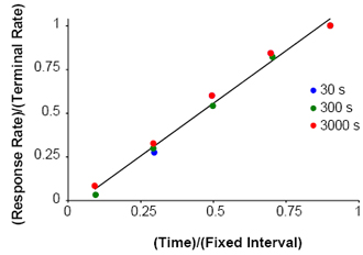
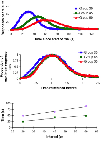
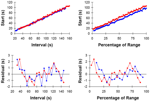
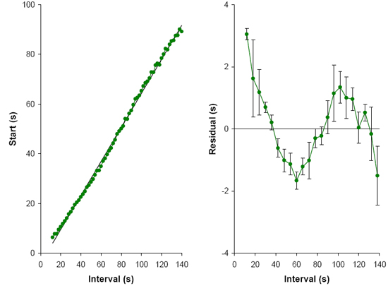
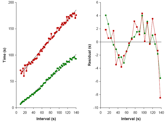
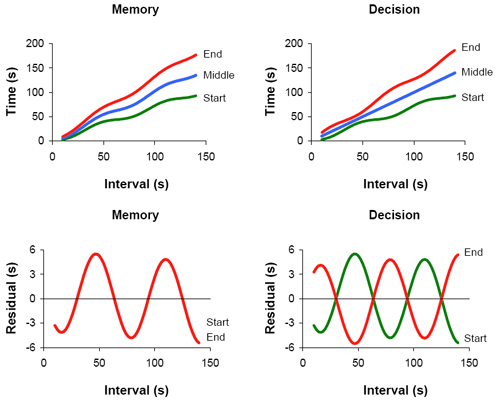
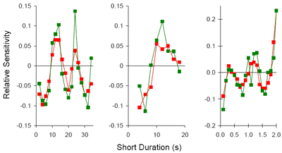
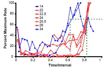
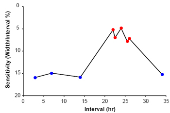
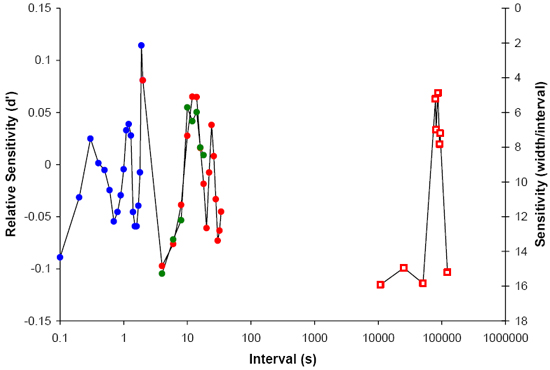
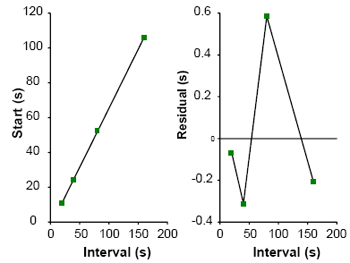
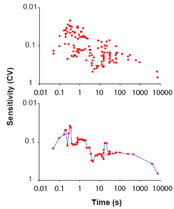
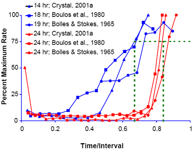
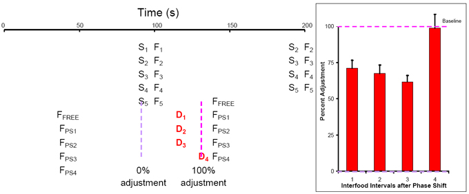
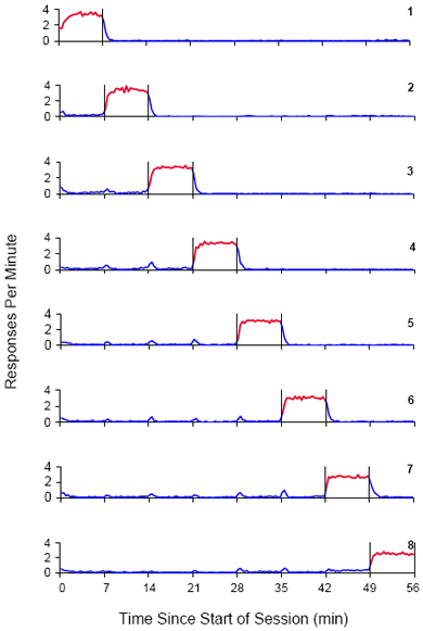
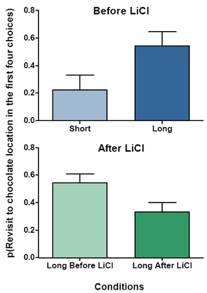
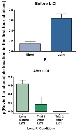
Supported by a grant from the National Institute of Mental
Health (MH64799) to J.D.C. I thank Kenneth W. Maxwell for assistance with reanalyzing published data.
|